
Advanced Excel Tutorial
The most widely used business software in the world is Microsoft Excel. This MS Excel tutorial will walk you through some of the most useful ideas and techniques to help you master MS Excel’s potential and surprise your coworkers.
Interface Navigation
An effective first step to becoming proficient in Excel is its user interface. Let’s start with the basics. The Tab key can be used to advance to the subsequent cell in the right-hand column while entering data into Excel.
To proceed to the cell in the subsequent row, press the Enter key. Pressing Enter will return you to the cell in the column you started after moving across the columns with the tab key.
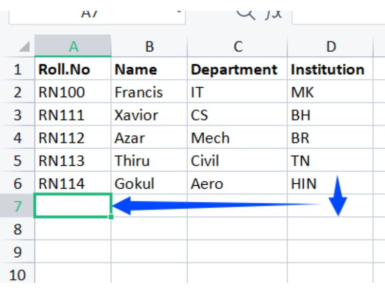
The last used cell in that direction can be reached by simultaneously pressing the Ctrl key and the Up, Down, Left, or Right directional arrow keys.
To navigate lengthy lists, this is quite helpful. You can access the first cell in your data range by simultaneously pressing the Ctrl and Home keys.
Proficiency with Shortcuts
Learning some practical keyboard, mouse, and touchpad shortcuts is the best approach to speeding up your daily Excel work.
Start by becoming familiar with the standard keyboard shortcuts if you’re a beginner. Ctrl + C and Ctrl + V are useful shortcuts to learn for copying and pasting. Then Ctrl + Z to undo the previous action.
Push yourself to learn more as you start utilizing these quick cuts in your regular work.
Excel features more than 500 keyboard shortcuts and a huge number of helpful tips for accelerating your work. Even though you won’t use all of them, it’s a good idea to master a few to make using Excel simpler.
Freeze Panes
As you scroll around the spreadsheet, this fantastic feature ensures that your headers and other labels remain visible at all times. It is a crucial Excel ability to possess.
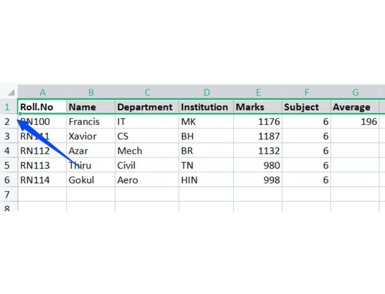
Typically, the top row of a spreadsheet only contains the headings. Therefore, select
View > Freeze Panes > Freeze Top Row to freeze this region.
The headings are still visible on the screen, even if we are looking at a particular row in the screenshot below.
As many columns and rows as necessary may be frozen.
The first cell after the rows and columns you want to freeze should be clicked. Click on cell B4 to freeze three rows and one column, for instance.
Now, click View → Freeze Panes → Freeze to Row 1 and Column A
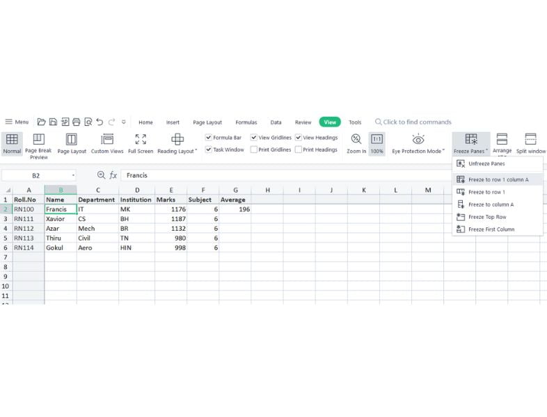
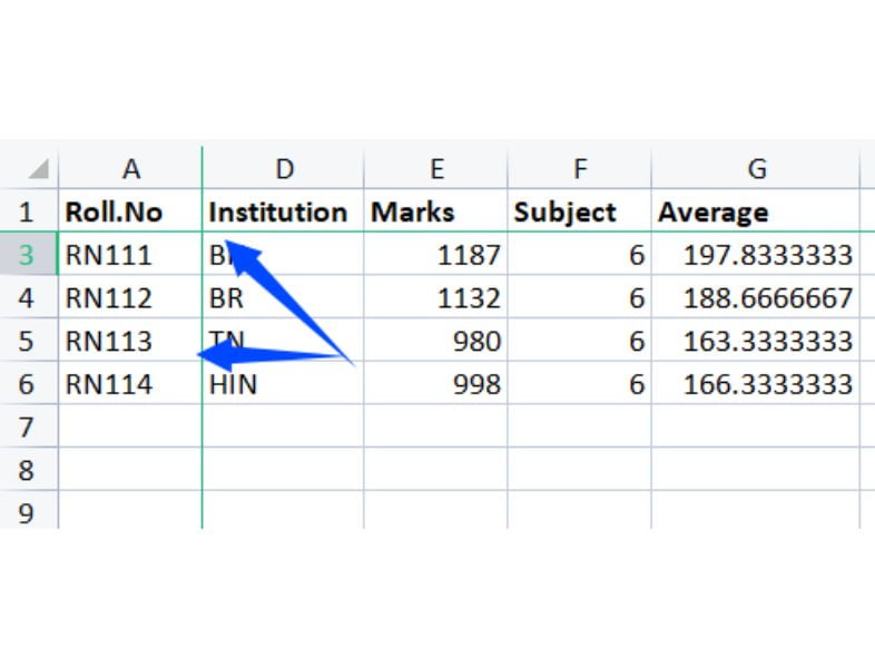
The first three rows are still visible as you scroll down at this time. Column A is still visible when you scroll to the right.
Mastery of Excel Formulas
Being proficient at writing formulas is one of the key components of mastering Excel. These are Excel’s muscles.
If you possess this ability, you will be head and shoulders above the competition, whether you are utilizing simple formulas or more complex ones to accomplish calculations in cells.
- Start by creating simple calculations that add, subtract, multiply, and divide quantities if you are unfamiliar with formulas.
- Then start becoming familiar with some of the more widely utilized functions. SUM, IF, VLOOKUP, COUNTIF, and CONCATENATE are a few of these.
- You are capable of doing practically anything once you feel at ease creating formulas.
- Charts, conditional formatting rules, and other Excel features can all be strengthened by the use of formulas.
Learn to Utilize the drop-down List Facility
An easy-to-use drop-down list on a spreadsheet may greatly simplify text entry and, more significantly, guarantee its accuracy.
To create a drop-down menu,
Step 1: Choose the range of cells in which the list should be displayed.
Step 2: Select Data > Insert Drop-Down List.
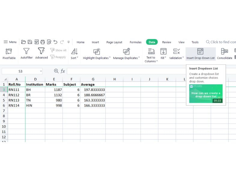
Step 3: From the Allow list, choose List.
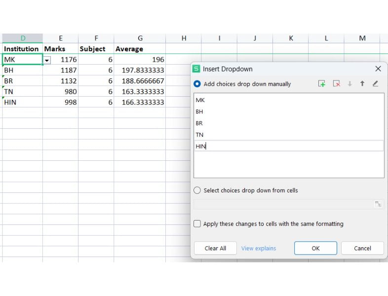
Step 4: After that, either manually enter the list items in the source field, comma-separating each one. Instead, select a set of cells that contain the list items.
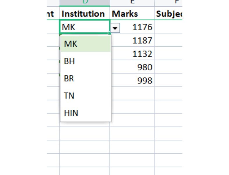
Now that you have a drop-down list, entering data is quick and accurate.
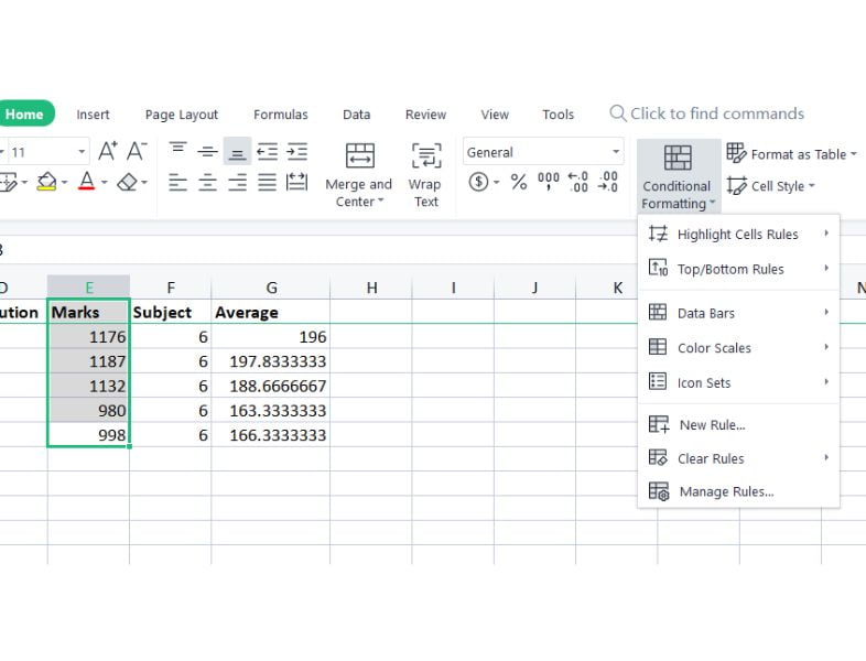
Learn to visualize key data with conditional formatting
One of the most commonly used Excel capabilities is conditional formatting. It makes it possible for the user to swiftly understand the information they are reading.
Simple criteria can be set up to format cells automatically when a goal is achieved, a deadline has passed, or perhaps sales have fallen below a predetermined level.
For a simple illustration, let’s say we want to make the cell green if the value is greater than 300.
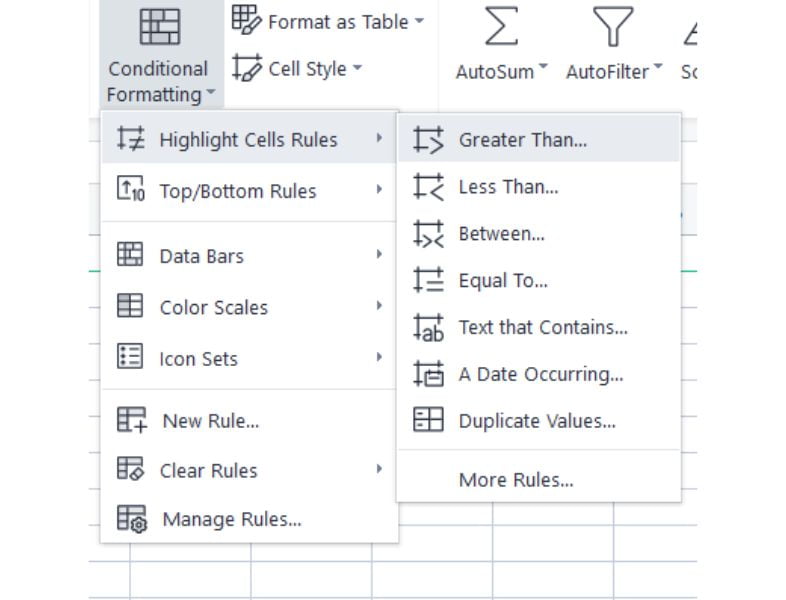
- Select the cell range that will get conditional formatting.
- Select Greater Than under Home > Conditional Formatting > Highlight Cell Rules.
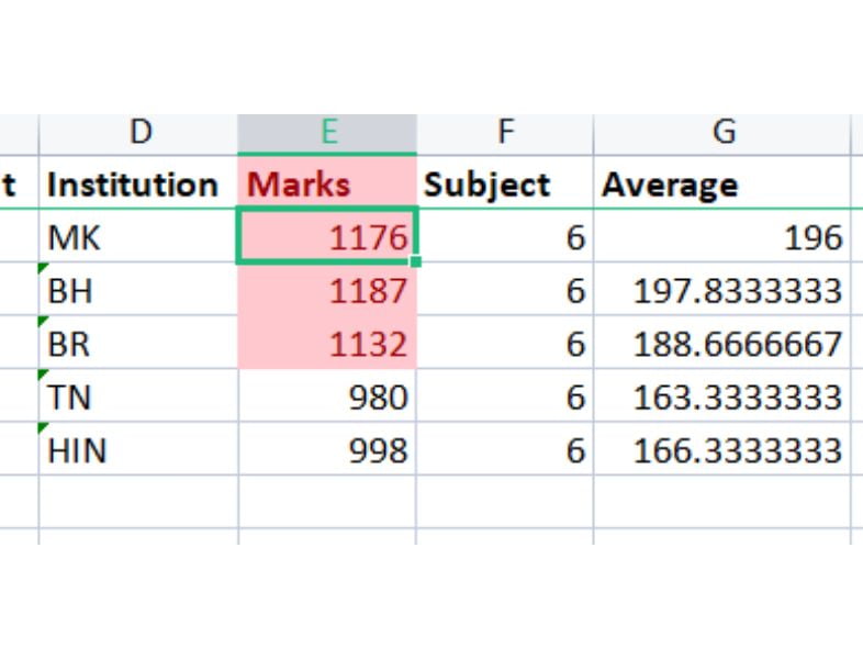
Although here, a light red fill and dark red text are employed, there are many other formatting alternatives.
Applying data bars and icon sets is also possible with conditional formatting. These images have a lot of power.
Data bars applied to the same range of values are displayed in the image below.
Flash Fill
A fantastic feature that manipulates data quickly is called Flash Fill. With the help of this functionality, routine data purification tasks that previously required the use of formulas and macros may be completed much more quickly.
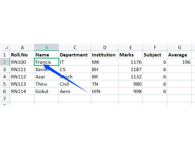
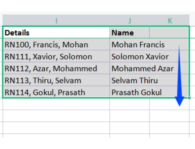
Consider the list that follows. The name from the list in column A should be extracted.

As you type, Flash Fill notices a pattern in your behavior and asks if you want it repeated throughout the remaining rows. Enter the first name in cell B2 and the second name in cell B3. This is incredible!
Once you hit Enter, the data will be extracted.
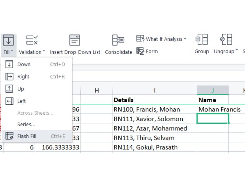
There are various approaches to using Flash Fill. The button is also located on the Ribbon’s Data tab, and you may access it by pressing Ctrl + E.
Summarize Data with Pivot Tables
One of Excel’s most outstanding features is the pivot table. Large dataset summarization is as simple as 1, 2, and 3.
To segment, a lengthy list of sales and view sales by region or even sales of certain products in each region, utilize a pivot table.
They are not only very easy to use but also very powerful. A pivot table is a tool that simplifies the report-creation process and eliminates the need for complicated calculations.
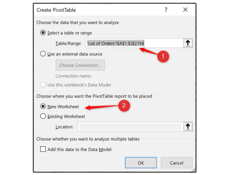
Creating a pivot table
Step 1: Select the list of data you wish to summarize by clicking.
Step 2: Select PivotTable under Insert.
Step 3: Select whether you want the pivot table to be a new or existing worksheet in the Create PivotTable window, and check that the range being utilized is right.
Step 4: To create your PivotTable, drag and drop fields from the field list into the four spaces.
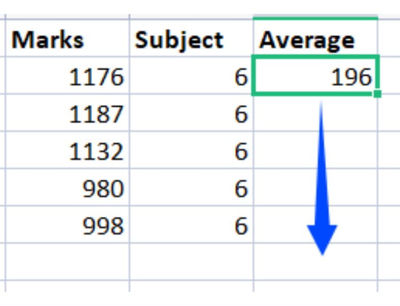
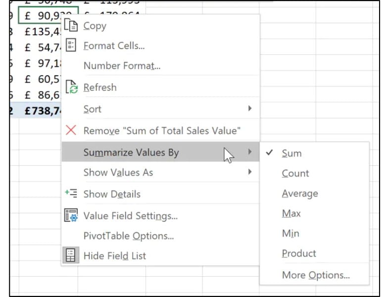
The product category is shown in rows, the years are listed in columns, and the values section shows the total sales amount.
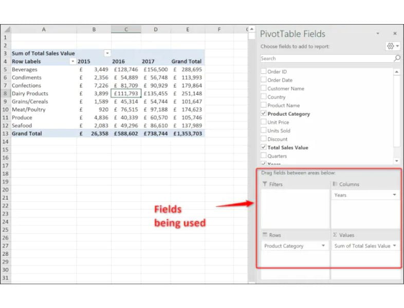
Calculations like sum, count, and average are carried out in the Values area.
By selecting Summarize Values By from the context menu when you right-click a PivotTable value and then the desired function, you may alter the calculation.
Pivot tables have a lot more features, but they are outside the scope of this article.
Grab some spreadsheet data, insert a pivot table, and start dragging fields into the sections to explore the options with pivot tables. It’s true that you only learn a tool by using it.
Protecting Excel Data
If the data is accurate, Excel features like pivot tables, formulas, and conditional formatting will function properly.
Some of the suggestions in this article show how to keep this accuracy, such as making drop-down menus and using Flash Fill.
Another critical action to take is to protect your Excel data.
The most common sort of protection in Excel is to safeguard the sheet, though there are other types as well.
Two steps are involved in protecting a sheet.
- You must first specify which worksheet cells you do not want to lock.
- Users can still edit these cells as a result of this. You then apply the defense.
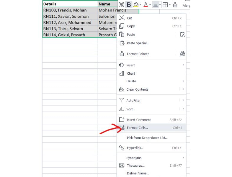
Step 1: Choose the cell range(s) you want to unlock (hold down the Ctrl key to select multiple ranges at the same time).
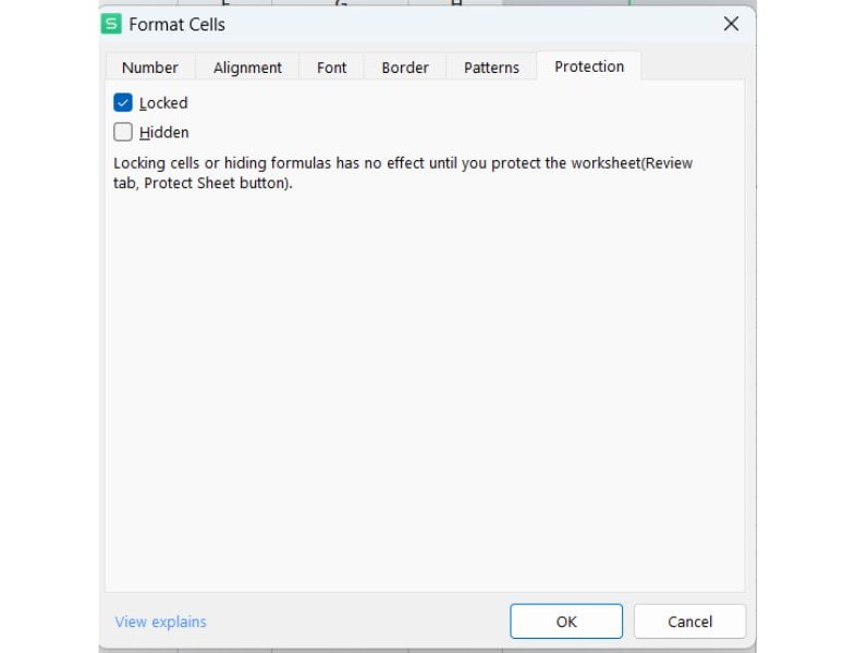
Step 2: To see the Format Cells dialogue, press Ctrl + 1.
Step 3: Uncheck the locked box under the Protection tab, then click OK.
Step 4: Select Protect Sheet under Review.
Step 5: For further security, you can enter a password, but doing so is optional (this is typically omitted as you are normally protecting against accidents and a password is unnecessary).
Step 6: Click “OK” after checking the boxes next to any functionality consumers will need to use.
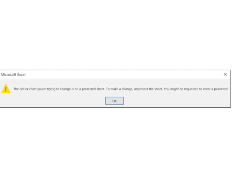
Still changeable, but with restricted utility, are the unlocked cells. A notification informing you that the sheet is protected will show up if you attempt to edit a locked cell.
Boost your efficiency using Power Query and Power Pivot
Knowing how to use these two Power Tools will elevate you above the average user.
- Data import and shaping tools like Power Query are used to prepare data for analysis. It may be found on the Ribbon’s Data tab.
- You may simply import data with Power Query from a wide range of (constantly evolving) sources, including CSV, the web, and folders.
- After that, the Power Query Editor offers a user-friendly setting for a variety of cleaning and shaping tasks like separating columns, formatting, deleting duplicates, and unpivoting data.
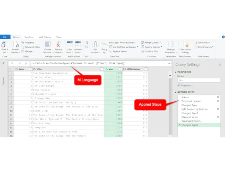
- M is the name of the language that Power Query uses. Although challenging to learn, 99% of Excel users do not require this.
- The editor provides all the features a user would need.
- Each modification is saved as a step that can later be refreshed with the push of a button.
- Power Pivot, commonly referred to as the data model, is a tool that makes it possible to store enormous amounts of data.
- We can move past Excel’s physical constraints by storing data in Power Pivot.
- In this, you can create DAX functions and associations between different data tables.
- You can get much more power from these models and the use of DAX than you can from a spreadsheet.
- Anyone who has to undertake complex analysis or is involved in evaluating vast amounts of data should be aware of this tool.
Create Macros with VBA
You can increase your productivity by automating repetitive operations with macros.
These tasks can be difficult, but for the majority of users, they are routine repetitions of quite easy tasks. To complete the jobs more quickly and accurately, use macros.
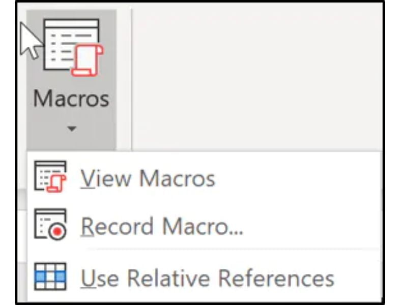
By videotaping yourself using Excel, you can begin using macros. This will create a macro and generate the VBA code. On the Ribbon’s View tab, you’ll discover the macro recorder. That button is the final one.
- You and your coworkers can save a tonne of time by recording macros.
- You can edit your macros if you want to go further by learning Excel VBA.
- With VBA, you may add functionality to your macros that goes much beyond simple recording and that Excel does not naturally provide.
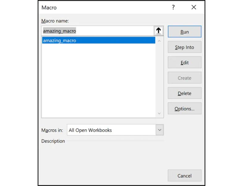
- Seeing the VBA code that was generated by a recording;
- Select the macro from the list by choosing View > Macros, then click Edit.
Conclusion
We hope this Advanced Excel Tutorial will help you get started with Excel mastery. The ideal approach to learning Excel is to enroll in our best MS Excel training in Chennai, which teaches you everything you need to know and puts your knowledge into practice at SLA.